Dynamic analysis in zebrafish neural crest development

This tutorial provides a step-by-step workflow for analyzing transcriptional dynamics in our newly sequenced zebrafish Smart-seq3 dataset, focused on neural crest cell development. Leveraging state-of-the-art tools such as scvelo [Bergen et al., 2020, La Manno et al., 2018] and cellrank [Lange et al., 2022, Weiler et al., 2024, Reuter et al., 2019], this guide centers on the use of the regvelo package to model RNA velocity with gene regulatory priors.

We walk through the complete pipeline, from data preprocessing to model training and transcription factor perturbation analysis. The goal is to uncover key regulators and dynamic processes shaping neural crest development, providing a reproducible framework for applying regvelo to similar single-cell transcriptomics studies.

Library import

import numpy as np
import pandas as pd
import scanpy as sc
import scvelo as scv
import torch

import cellrank as cr
import scvi

import mplscience
import matplotlib.pyplot as plt
import seaborn as sns

from regvelo import REGVELOVI
import regvelo as rgv

scvi.settings.seed = 0

scv.settings.verbosity = 3
cr.settings.verbosity = 2

%matplotlib inline

plt.rcParams["svg.fonttype"] = "none"
scv.settings.set_figure_params("scvelo", dpi=100, transparent=True, fontsize=14, color_map="viridis")

Define functions and constants

SIGNIFICANCE_PALETTE = {"n.s.": "#dedede", 
                        "*": "#90BAAD", 
                        "**": "#A1E5AB", 
                        "***": "#ADF6B1"}

from anndata import AnnData
from typing import Sequence

def visits_diff_perTF(adata: AnnData, 
                      terminal_state: str | Sequence[str], 
                      dd_sig: np.ndarray, 
                      sig_palette: dict) -> list[pd.DataFrame, list[str]]:

    data = []
    palette_rel = []
    
    for i in range(len(TERMINAL_STATES)):
        ts = TERMINAL_STATES[i]
        p_value = dd_sig[i]
        terminal_indices_sub = np.where(adata.obs["term_states_fwd"].isin([ts]))[0]
    
        values = adata.obs["visits_diff"].iloc[terminal_indices_sub]
        subgroups = [ts]*len(values)
    
        for val, subgrp in zip(values, subgroups):
            data.append({"Value": val, "Group": subgrp})
    
        significance = rgv.mt.get_significance(p_value)
        print(f"{ts}: {p_value}")
        palette_rel.append(SIGNIFICANCE_PALETTE[significance])
    
    return pd.DataFrame(data), palette_rel

def plot_visits_dist(df: pd.DataFrame, palette_rel: list[str], tick_range: float) -> None:
    with mplscience.style_context():
        sns.set_style("whitegrid")
        fig, ax = plt.subplots(figsize=(3, 3))
        
        sns.boxplot(
            data=df,
            y="Group",
            x="Value",
            palette=palette_rel,
            ax=ax,
            flierprops={
                'marker': '.',
                'markersize': 5,
                'markerfacecolor': 'black',
                'markeredgecolor': 'black'
            }
        )
        ax.set_xlabel("Density change likelihood")
        ax.set_ylabel("Terminal state")
    
        tick_range = tick_range
        tick_step = tick_range
        xmin, xmax = 0.5 - tick_range, 0.5 + tick_range
    
        ticks = np.arange(xmin, xmax + 1e-6, tick_step)
        if 0.5 not in ticks:
            ticks = np.sort(np.append(ticks, 0.5))
        
        ax.set_xlim(xmin, xmax)
        ax.set_xticks(ticks)
        
        for spine in ax.spines.values():
            spine.set_visible(True)
    
        plt.show()

Load data

adata = rgv.datasets.zebrafish_nc()
prior_net = rgv.datasets.zebrafish_grn()
TF_list = adata.var_names[adata.var["is_tf"]].tolist()

sc.pp.neighbors(adata, n_neighbors=30, n_pcs=50)
scv.pp.moments(adata)

---------------------------------------------------------------------------
AttributeError                            Traceback (most recent call last)
AttributeError: 'MessageFactory' object has no attribute 'GetPrototype'

---------------------------------------------------------------------------
AttributeError                            Traceback (most recent call last)
AttributeError: 'MessageFactory' object has no attribute 'GetPrototype'

---------------------------------------------------------------------------
AttributeError                            Traceback (most recent call last)
AttributeError: 'MessageFactory' object has no attribute 'GetPrototype'

---------------------------------------------------------------------------
AttributeError                            Traceback (most recent call last)
AttributeError: 'MessageFactory' object has no attribute 'GetPrototype'

---------------------------------------------------------------------------
AttributeError                            Traceback (most recent call last)
AttributeError: 'MessageFactory' object has no attribute 'GetPrototype'

computing moments based on connectivities
    finished (0:00:00) --> added 
    'Ms' and 'Mu', moments of un/spliced abundances (adata.layers)

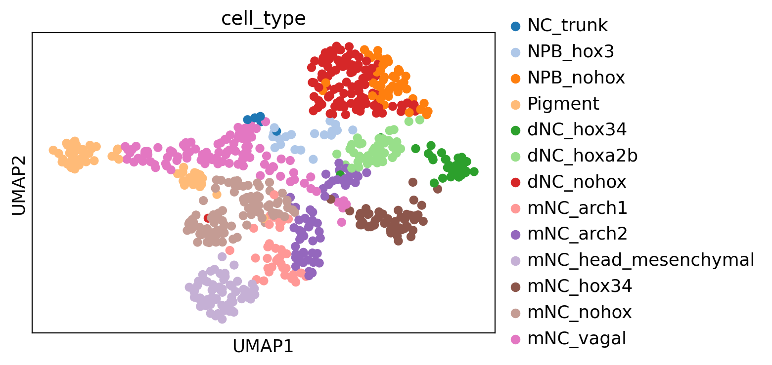
sc.pl.umap(adata, color='cell_type', palette=sc.pl.palettes.vega_20)

Preprocessing

adata = rgv.pp.preprocess_data(adata)
adata = rgv.pp.set_prior_grn(adata, prior_net.T)

computing velocities
    finished (0:00:00) --> added 
    'velocity', velocity vectors for each individual cell (adata.layers)

TF_list = set(TF_list).intersection(adata.var_names)
TF_list = list(TF_list)
print("final number of TFs: " + str(len(TF_list)))

final number of TFs: 81

W = adata.uns["skeleton"].copy()
W = torch.tensor(np.array(W))

sparsity = W.sum() / ((W.sum(1) != 0).sum() * W.shape[0])
print("network sparsity: " + str(np.array(sparsity)))

network sparsity: 0.052775327

Train RegVelo model

REGVELOVI.setup_anndata(adata, spliced_layer="Ms", unspliced_layer="Mu")
reg_vae = REGVELOVI(adata, W=W.T, regulators=TF_list, soft_constraint=False)

reg_vae.train()

Monitored metric elbo_validation did not improve in the last 45 records. Best score: -2377.829. Signaling Trainer to stop.

adata = reg_vae.add_regvelo_outputs_to_adata(adata=adata)
scv.tl.velocity_graph(adata)

computing velocity graph (using 1/128 cores)
    finished (0:00:00) --> added 
    'velocity_graph', sparse matrix with cosine correlations (adata.uns)

Predict terminal states

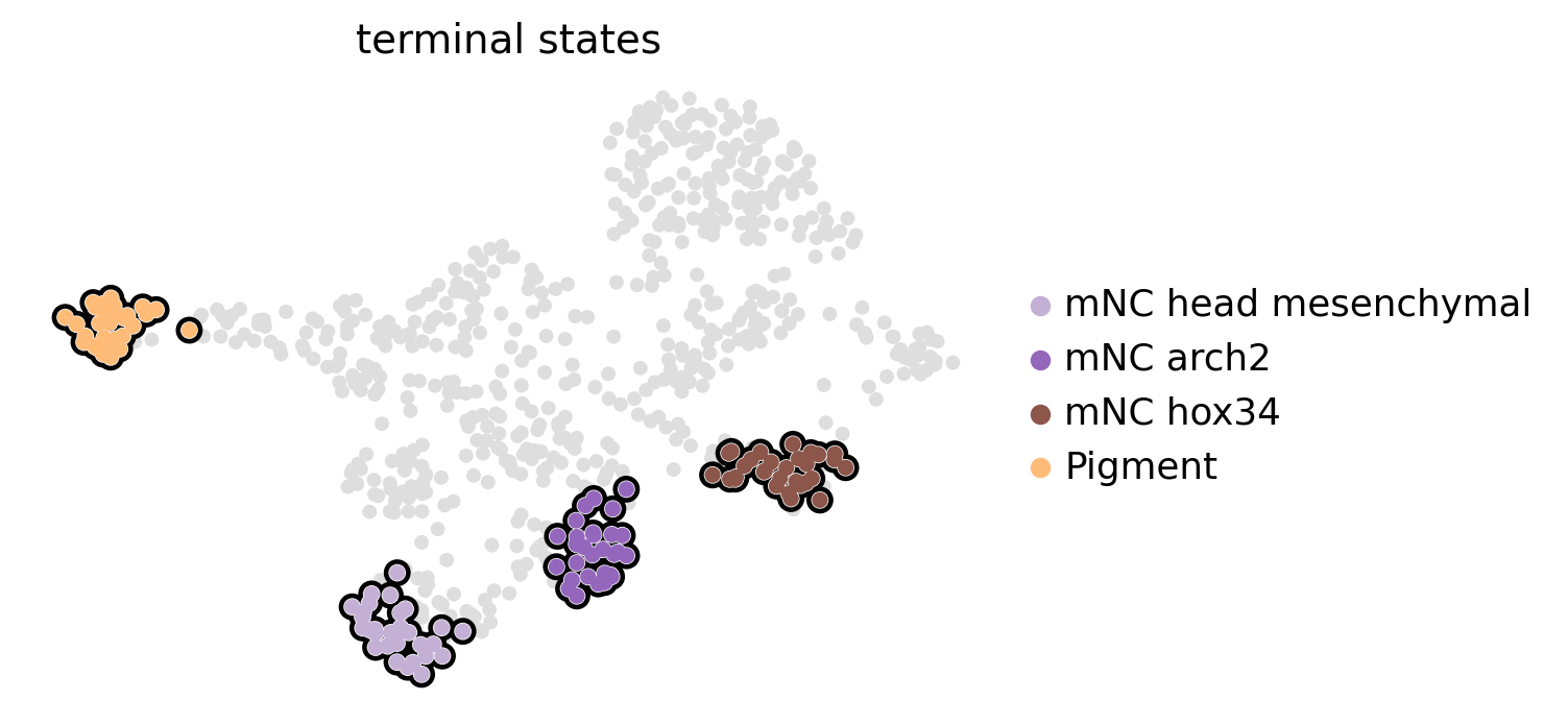
TERMINAL_STATES = ["mNC_head_mesenchymal",
                  "mNC_arch2",
                  "mNC_hox34",
                  "Pigment"]
vk = cr.kernels.VelocityKernel(adata).compute_transition_matrix()
estimator = cr.estimators.GPCCA(vk)

## evaluate the fate prob on original space
estimator.compute_macrostates(n_states=7, cluster_key="cell_type")
estimator.set_terminal_states(TERMINAL_STATES)
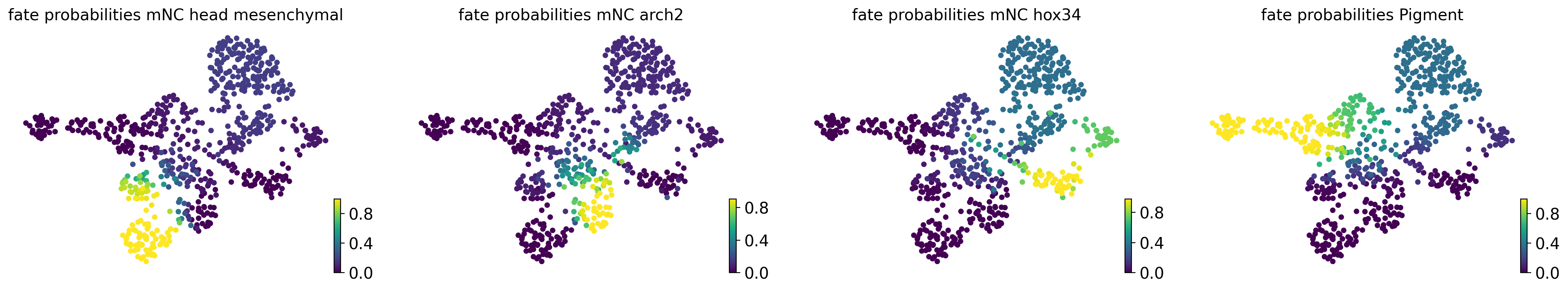
estimator.compute_fate_probabilities()
estimator.plot_fate_probabilities(same_plot=False)

Computing transition matrix using `'deterministic'` model
Using `softmax_scale=9.5760`
    Finish (0:00:07)
Computing Schur decomposition
Adding `adata.uns['eigendecomposition_fwd']`
       `.schur_vectors`
       `.schur_matrix`
       `.eigendecomposition`
    Finish (0:00:07)
Computing `7` macrostates
Adding `.macrostates`
       `.macrostates_memberships`
       `.coarse_T`
       `.coarse_initial_distribution
       `.coarse_stationary_distribution`
       `.schur_vectors`
       `.schur_matrix`
       `.eigendecomposition`
    Finish (0:00:00)
Adding `adata.obs['term_states_fwd']`
       `adata.obs['term_states_fwd_probs']`
       `.terminal_states`
       `.terminal_states_probabilities`
       `.terminal_states_memberships
    Finish`
Computing fate probabilities
Adding `adata.obsm['lineages_fwd']`
       `.fate_probabilities`
    Finish (0:00:00)

estimator.plot_macrostates(which="terminal", legend_loc="right", s=100)

Save model

reg_vae.save("rgv_model")

Perform perturbation screening

In the perturbation screening step, RegVelo enables users to generate a perturbed vector field matrix, which is stored in adata_target_perturb.layers["velocity"]. This is then used to construct a new CellRank kernel, which results in an updated estimate of perturbed cell fate prpobabilities.

We evalute the perturbation effects using two approaches:
(a) by comparing cell fate probabilities before and after perturbation, and
(b) by simulating cell transitions using a Markov chain based on transition matrices inferred from the velocity fields of the unperturbed and perturbed systems.

Let \(m\) denote the number of terminal states and \(N_C\) the number of cells. For approach (a), we define the depletion likelihood to a terminal state \(k\) as the normalized Mann-Whitney \(U\) statistic

(1)\[\begin{equation} l_d = \frac{1}{N_c^2} \sum_{n=1}^{N_C} \sum_{n^*=1}^{N_C} \mathbb{I} (\Pi_{:,k}(n) > \Pi_{:,k}^*(n^*)), \end{equation}\]

where \(\mathbb{I}\) is the indicator function and \(\Pi, \ \Pi^* \in \mathbb{R}^{N_c \times m}\) are the control and perturbed cell fate probability matrices, respectively. For a terminal state \(k\), a depletion likelihood \(l_d > 0.5\) indicates a long-term depletion effect in the perturbed system, as illustrated in Figure 1 (a).

It is important to note that the depletion likelihood depends on the long-term fate probabilities of transient cells. In particular, a reduction in a transient cell’s probability of reaching one terminal state must be balanced by an increase in its probability of reaching other terminal states, since the row-wise sums of \(\Pi\) and \(\Pi^*\) are approximately 1. This redistribution can thus lead to possible long-term enrichment effects in terminal states.

To capture short-term dynamics of the perturbed system, we also simulate the development of progenitor cells over a finite number of steps (n_steps) using Markov chain derived from the velocity-based transition matrices of both control and perturbed systems using the function rgv.tl.markov_density_simulation. We then compare the frequency with which terminal cells are reached in both cases, quantifying depletion effects in short-term dynamics (Figure 1(b)).

The Markov chain simulations can be run with either method='stepwise' (default) or method='one-step'. The stepwise method simulates transitions one step at a time and terminates each trajectory either upon reaching a terminal cell or after n_steps, whichever comes first. In contrast, the one-step method computes the cell state distribution after n_steps and draws samples directly from this distribution, without modeling intermediate transitions.

Figure 1: Visualization of perturbation effects.
(a) Depletion likelihood \(l_d\) where \(\bar{\Pi}_{.k}\) and \(\bar{\Pi}^*_{.k}\) denote mean cell fate probabilities.
(b) Simulated Markov chain transitions of progenitor cells.

In the following, we demonstrate both perturbation quantification approaches for two perturbed models, in which we remove the transcription factors nr2f5 and elf1, respectively.

Terminal states for the perturbed dynamics can be defined in two ways: Either by explicitly setting them via estimator.set_terminal_states(TERMINAL_STATES), or by reusing the terminal state indices identified in the original dynamics using CellRank.

Calculating depletion likelihood based on cell fate probability

adata_perturb_dict = {}
cand_list = ["nr2f5", "elf1"]

for TF in cand_list:
    model = 'rgv_model'
    adata_target_perturb, reg_vae_perturb =  rgv.tl.in_silico_block_simulation(model=model,
                                                                               adata=adata,
                                                                               TF=TF,
                                                                               cutoff=0)
    adata_perturb_dict[TF] = adata_target_perturb

INFO     File rgv_model/model.pt already downloaded                                                                
INFO     File rgv_model/model.pt already downloaded

ct_indices = {
    ct: adata.obs["term_states_fwd"][adata.obs["term_states_fwd"] == ct].index.tolist()
    for ct in TERMINAL_STATES}

# Computing states transition probability for perturbed systems
for TF, adata_target_perturb in adata_perturb_dict.items():
    vkp = cr.kernels.VelocityKernel(adata_target_perturb).compute_transition_matrix()
    estimator = cr.estimators.GPCCA(vkp)
    estimator.compute_macrostates(n_states=7, cluster_key='cell_type')
    estimator.set_terminal_states(ct_indices)
    estimator.compute_fate_probabilities()

    adata_perturb_dict[TF] = adata_target_perturb

Computing transition matrix using `'deterministic'` model
Using `softmax_scale=9.9602`
    Finish (0:00:00)
Computing Schur decomposition
Adding `adata.uns['eigendecomposition_fwd']`
       `.schur_vectors`
       `.schur_matrix`
       `.eigendecomposition`
    Finish (0:00:00)
Computing `7` macrostates
Adding `.macrostates`
       `.macrostates_memberships`
       `.coarse_T`
       `.coarse_initial_distribution
       `.coarse_stationary_distribution`
       `.schur_vectors`
       `.schur_matrix`
       `.eigendecomposition`
    Finish (0:00:00)
Adding `adata.obs['term_states_fwd']`
       `adata.obs['term_states_fwd_probs']`
       `.terminal_states`
       `.terminal_states_probabilities`
       `.terminal_states_memberships
    Finish`
Computing fate probabilities
Adding `adata.obsm['lineages_fwd']`
       `.fate_probabilities`
    Finish (0:00:00)
Computing transition matrix using `'deterministic'` model
Using `softmax_scale=9.6380`
    Finish (0:00:00)
Computing Schur decomposition
Adding `adata.uns['eigendecomposition_fwd']`
       `.schur_vectors`
       `.schur_matrix`
       `.eigendecomposition`
    Finish (0:00:00)
Computing `7` macrostates
Adding `.macrostates`
       `.macrostates_memberships`
       `.coarse_T`
       `.coarse_initial_distribution
       `.coarse_stationary_distribution`
       `.schur_vectors`
       `.schur_matrix`
       `.eigendecomposition`
    Finish (0:00:00)
Adding `adata.obs['term_states_fwd']`
       `adata.obs['term_states_fwd_probs']`
       `.terminal_states`
       `.terminal_states_probabilities`
       `.terminal_states_memberships
    Finish`
Computing fate probabilities
Adding `adata.obsm['lineages_fwd']`
       `.fate_probabilities`
    Finish (0:00:00)

df = rgv.mt.cellfate_perturbation(perturbed=adata_perturb_dict, baseline=adata, terminal_state=TERMINAL_STATES)
df

	Depletion likelihood	p-value	FDR adjusted p-value	Terminal state	TF
0	0.570827	0.000002	0.000009	mNC_head_mesenchymal	nr2f5
1	0.468141	0.980279	0.995731	mNC_arch2	nr2f5
2	0.459316	0.995731	0.995731	mNC_hox34	nr2f5
3	0.478670	0.916038	0.995731	Pigment	nr2f5
0	0.470181	0.973052	0.993760	mNC_head_mesenchymal	elf1
1	0.461354	0.993760	0.993760	mNC_arch2	elf1
2	0.467785	0.981355	0.993760	mNC_hox34	elf1
3	0.546538	0.001313	0.005252	Pigment	elf1

rgv.pl.cellfate_perturbation(adata=adata,
                             df=df,
                             fontsize=14,
                             figsize=(8, 4),
                             legend_loc='center left',
                             legend_bbox=(1.02, 0.5),
                             color_label="cell_type")

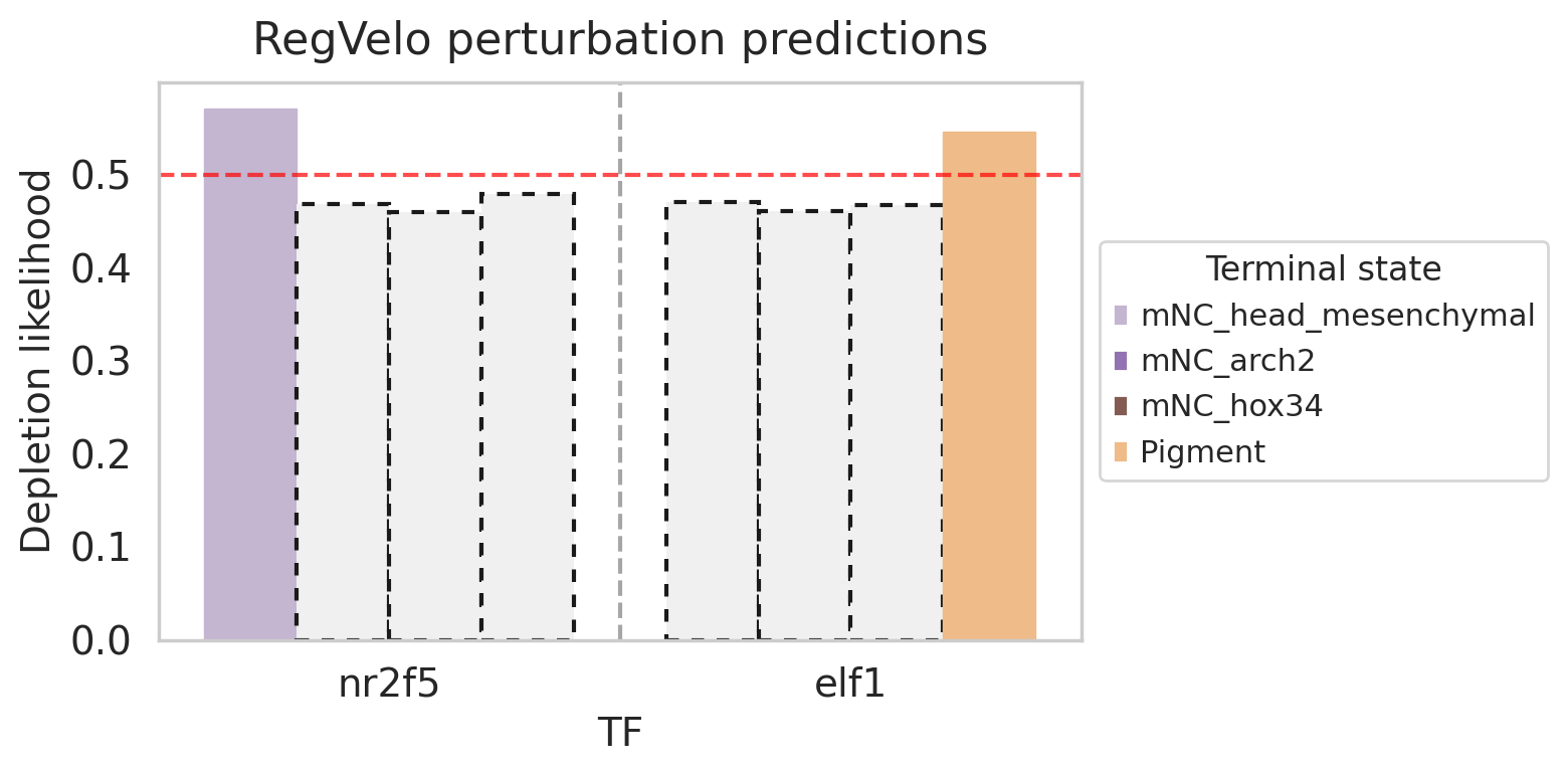
By removing the TF nr2f5, one would expect a depletion of the cell type mNC_head_mesenchymal and an enrichment of the cell types mNC_arch2, mNC_hox34, and Pigment in the long run, compared to the control dynamics.

By removing the TF elf1, one would expect a depletion of the cell type Pigment and an enrichment of the cell types mNC_head_mesenchymal, mNC_arch2, and mNC_hox34 in the long run, compared to the control dynamics.

For both models, we now have a look at their short-term perturbation effects and demonstrate both stepwiseand one-step methods. Transition matrices are computed using CellRank on the original and perturbed velocity fields.

Calculating density change likelihood based on stochastic simulations

For the Markov chain simulations, we note that the choice of n_steps in rgv.tl.markov_density_simulation can be made by evaluating the proportion of processes ending in a terminal cell using the control (unperturbed) cell state transition matrix. In this tutorial, we will use the default value n_steps=100.

The function additionally takes as input n_simulations, which determines the number of simulations to be performed for each cell. In this notebook, we will use the default value n_simulations=1000.

For the initial state, we select cells of type NPB_nohox and determine the start_indices and terminal_indices, which are required as input for the rgv.tl.markov_density_simulation function.

To compare the number of times each terminal cell is visited in the perturbed versus the control model, we compute the difference:

(2)\[\begin{equation} \# \text{visits in perturbed model} - \# \text{visits in control model}. \end{equation}\]

The absolute and relative number of visits to each terminal cell are stored in .obs["visits"] and .obs["visits_dens"], respectively.

For each terminal state, we then use the function rgv.tl.simulated_density_diff to compute the average difference in visit counts between the perturbed and unperturbed systems. This function also performs a paired t-test (scipy.stats.ttest_rel) to assess whether the number of visits differ significantly between the two systems. The resulting p-values are returned as output.

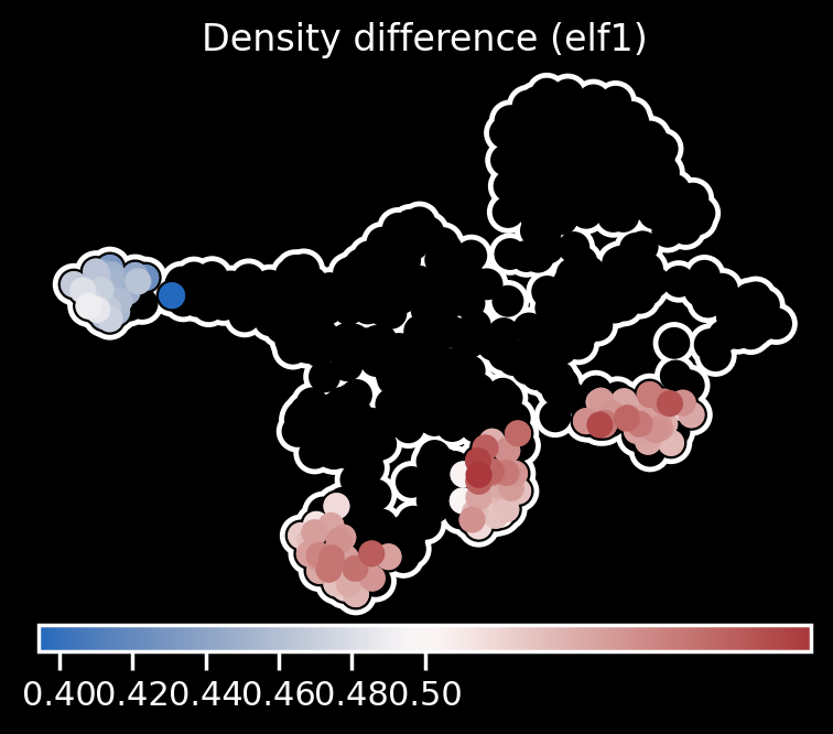
To visualize short-term perturbation effects, we use the function rgv.pl.simulated_density_diff. For each terminal cell, the function computes the difference in the number of visits between the perturbed and control simulations. To account for stochastic variability across simulations, this difference is scaled by \(1/\sqrt{\text{\# total simulations}}\). The resulting scaled differences are then passed through a sigmoid function and stored in adata.obs['visits_diff']. These scores are further smoothed over neighboring cells to produce a spatially coherent signal, stored in adata.obs['visits_diff_smoothed']. Values below 0.5 indicate a relative depletion of visits to the corresponding terminal cell under perturbation.

vk = cr.kernels.VelocityKernel(adata).compute_transition_matrix()
vkt = vk.transition_matrix.A
terminal_indices = np.where(adata.obs["term_states_fwd"].isin(TERMINAL_STATES))[0]
start_indices = np.where(adata.obs["cell_type"].isin(["NPB_nohox"]))[0]

Computing transition matrix using `'deterministic'` model
Using `softmax_scale=9.5760`
    Finish (0:00:00)

Method 1: Stepwise simulations - nr2f5 perturbation

We first consider the perturbed model by removing the TF nr2f5.

method = "stepwise"

TF = "nr2f5"
adata_perturb = adata_perturb_dict[TF].copy()
adata_perturb.obs["cell_type"] = adata.obs["cell_type"].copy()

vk_p = cr.kernels.VelocityKernel(adata_perturb).compute_transition_matrix()
vkt_p = vk_p.transition_matrix.A

Computing transition matrix using `'deterministic'` model
Using `softmax_scale=9.9602`
    Finish (0:00:00)

total_simulations = rgv.tl.markov_density_simulation(adata, 
                                                     vkt, 
                                                     start_indices, 
                                                     terminal_indices, 
                                                     TERMINAL_STATES,
                                                     method=method)

_ = rgv.tl.markov_density_simulation(adata_perturb, 
                                     vkt_p, 
                                     start_indices, 
                                     terminal_indices, 
                                     TERMINAL_STATES,
                                     method=method)

dd_score, dd_sig = rgv.tl.simulated_visit_diff(adata, adata_perturb, TERMINAL_STATES)
print(dd_score)
print(dd_sig)

[-79.1, -24.5, -41.400000000000006, -88.29999999999998]
[1.0388254084002412e-07, 6.385268221500673e-07, 6.971348452267312e-10, 0.0004889179271363851]

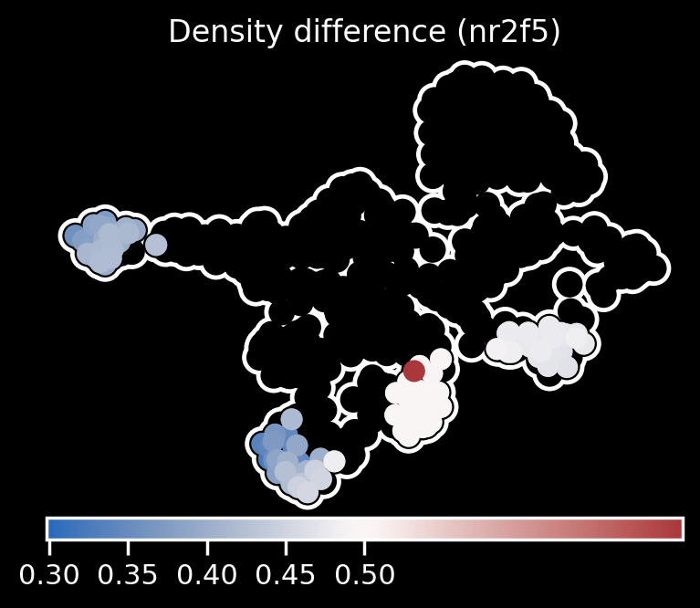
rgv.pl.simulated_visit_diff(adata, 
                            adata_perturb, 
                            TERMINAL_STATES, 
                            total_simulations,
                            title="Density difference (nr2f5)")

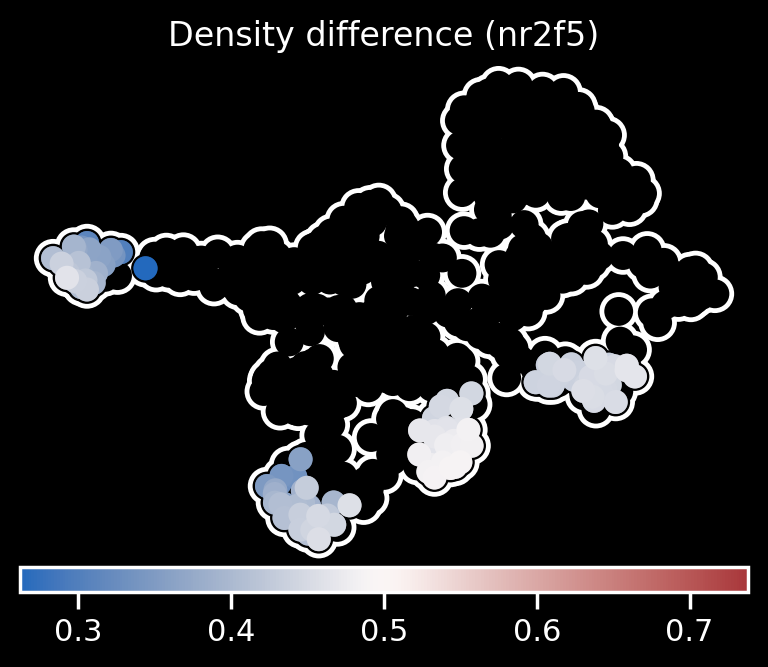
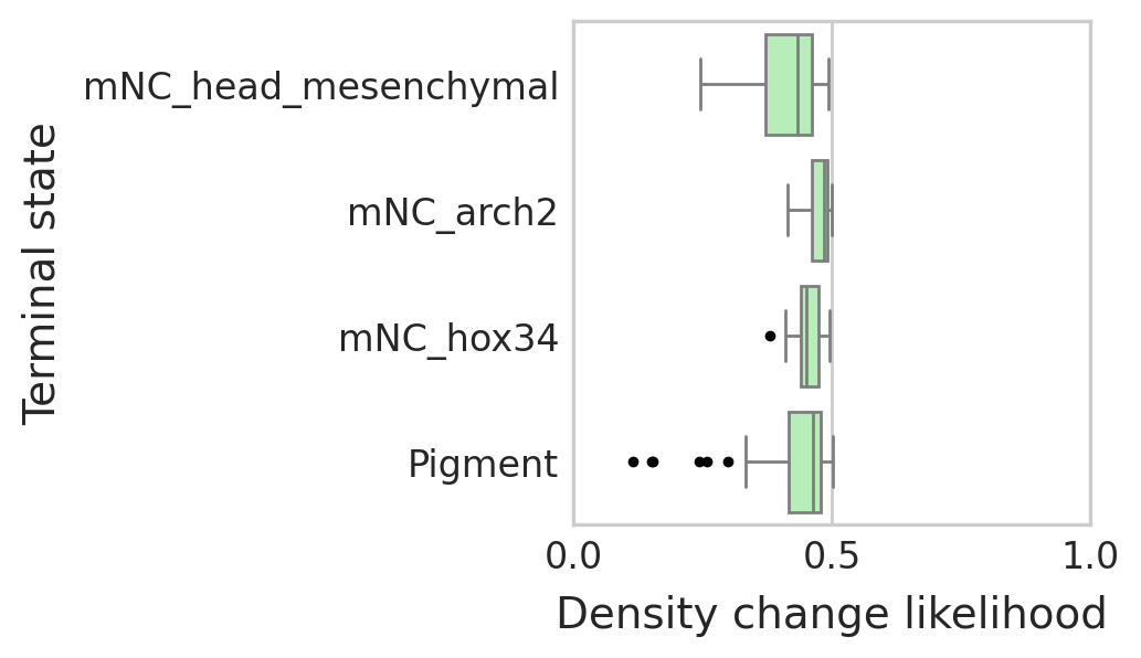
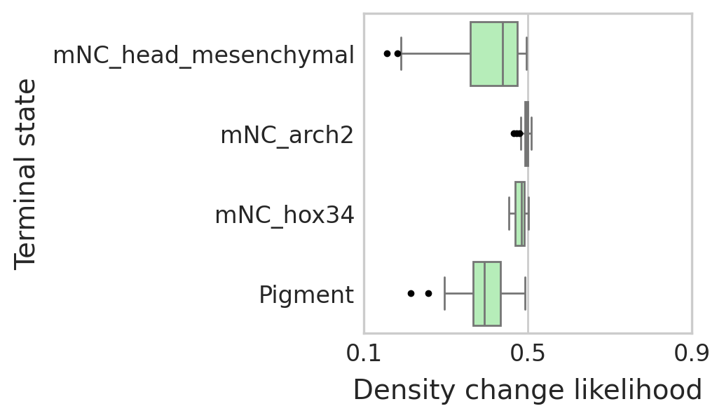
We also visualize the distribution of adata.obs['visits_diff'] for each terminal state using a boxplot. The values are grouped by terminal state and colored according to the p-value from the paired t-test comparing visit counts between the unperturbed and perturbed systems.

df, palette_rel = visits_diff_perTF(adata, TERMINAL_STATES, dd_sig, SIGNIFICANCE_PALETTE)

mNC_head_mesenchymal: 1.0388254084002412e-07
mNC_arch2: 6.385268221500673e-07
mNC_hox34: 6.971348452267312e-10
Pigment: 0.0004889179271363851

plot_visits_dist(df, palette_rel, 0.5)

Method 1: Stepwise simulations - elf1 perturbation

We now consider the perturbed model by removing the TF elf1.

del adata.obs['visits']
del adata.obs['visits_dens']
del adata.obs['visits_diff']
del adata.obs['visits_diff_smooth']

TF = "elf1"
adata_perturb = adata_perturb_dict[TF].copy()
adata_perturb.obs["cell_type"] = adata.obs["cell_type"].copy()

vk_p = cr.kernels.VelocityKernel(adata_perturb).compute_transition_matrix()
vkt_p = vk_p.transition_matrix.A

Computing transition matrix using `'deterministic'` model
Using `softmax_scale=9.6380`
    Finish (0:00:00)

total_simulations = rgv.tl.markov_density_simulation(adata, 
                                                     vkt, 
                                                     start_indices, 
                                                     terminal_indices, 
                                                     TERMINAL_STATES,
                                                     method=method)

_ = rgv.tl.markov_density_simulation(adata_perturb, 
                                     vkt_p, 
                                     start_indices, 
                                     terminal_indices, 
                                     TERMINAL_STATES,
                                     method=method)

dd_score, dd_sig = rgv.tl.simulated_visit_diff(adata, adata_perturb, TERMINAL_STATES)
print(dd_score)
print(dd_sig)

[4.900000000000006, 7.099999999999994, 5.36666666666666, -22.0]
[0.002008393908970593, 0.0008743624255374171, 0.004047887217802147, 0.013239451053673714]

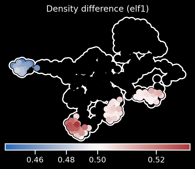
rgv.pl.simulated_visit_diff(adata, 
                            adata_perturb, 
                            TERMINAL_STATES, 
                            total_simulations,
                            title="Density difference (elf1)")

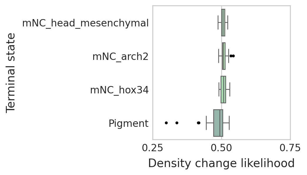
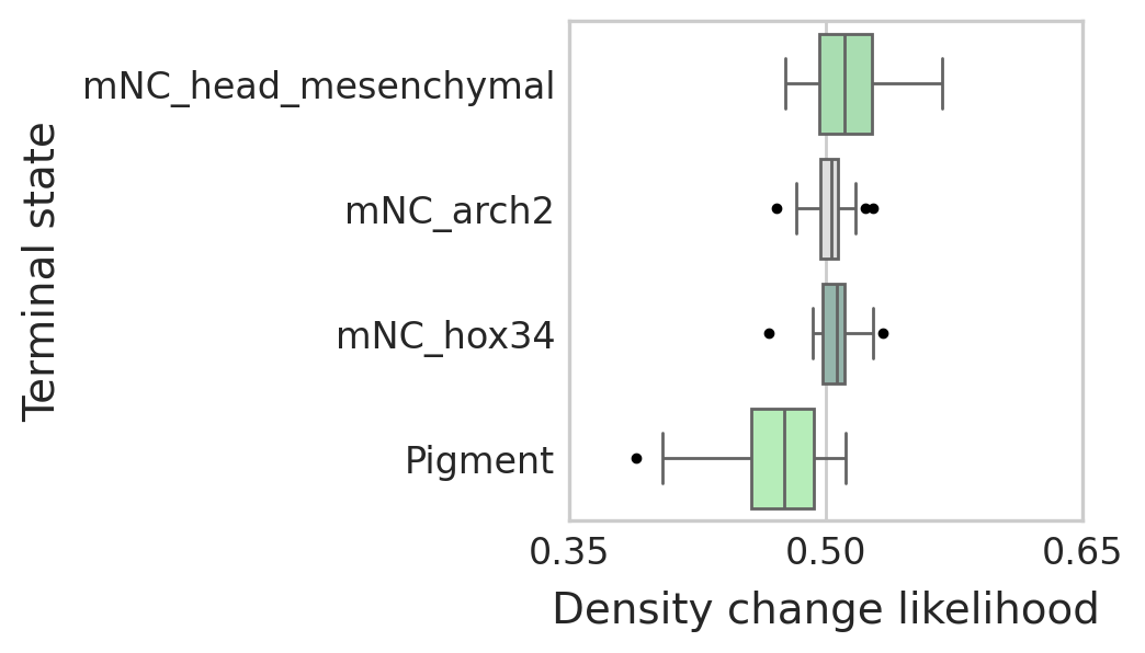
df, palette_rel = visits_diff_perTF(adata, TERMINAL_STATES, dd_sig, SIGNIFICANCE_PALETTE)

mNC_head_mesenchymal: 0.002008393908970593
mNC_arch2: 0.0008743624255374171
mNC_hox34: 0.004047887217802147
Pigment: 0.013239451053673714

plot_visits_dist(df, palette_rel, 0.25)

Method 2: One-step simulations - nr2f5 perturbation

del adata.obs['visits']
del adata.obs['visits_dens']
del adata.obs['visits_diff']
del adata.obs['visits_diff_smooth']

method = "one-step"

TF = "nr2f5"
adata_perturb = adata_perturb_dict[TF].copy()
adata_perturb.obs["cell_type"] = adata.obs["cell_type"].copy()

vk_p = cr.kernels.VelocityKernel(adata_perturb).compute_transition_matrix()
vkt_p = vk_p.transition_matrix.A

Computing transition matrix using `'deterministic'` model
Using `softmax_scale=9.9602`
    Finish (0:00:00)

total_simulations = rgv.tl.markov_density_simulation(adata, 
                                                     vkt, 
                                                     start_indices, 
                                                     terminal_indices, 
                                                     TERMINAL_STATES,
                                                     method=method)

_ = rgv.tl.markov_density_simulation(adata_perturb, 
                                     vkt_p, 
                                     start_indices, 
                                     terminal_indices, 
                                     TERMINAL_STATES,
                                     method=method)

dd_score, dd_sig = rgv.tl.simulated_visit_diff(adata, adata_perturb, TERMINAL_STATES)
print(dd_score)
print(dd_sig)

[-95.23333333333332, -4.600000000000001, -17.433333333333337, -95.46666666666667]
[1.8341934745831434e-05, 0.006290120629851753, 3.731241368483117e-08, 2.9413421676244866e-09]

rgv.pl.simulated_visit_diff(adata, 
                            adata_perturb, 
                            TERMINAL_STATES, 
                            total_simulations,
                            title="Density difference (nr2f5)")

df, palette_rel = visits_diff_perTF(adata, TERMINAL_STATES, dd_sig, SIGNIFICANCE_PALETTE)

mNC_head_mesenchymal: 1.8341934745831434e-05
mNC_arch2: 0.006290120629851753
mNC_hox34: 3.731241368483117e-08
Pigment: 2.9413421676244866e-09

plot_visits_dist(df, palette_rel, 0.4)

Method 2: One-step simulations - elf1 perturbation

del adata.obs['visits']
del adata.obs['visits_dens']
del adata.obs['visits_diff']
del adata.obs['visits_diff_smooth']

TF = "elf1"
adata_perturb = adata_perturb_dict[TF].copy()
adata_perturb.obs["cell_type"] = adata.obs["cell_type"].copy()

vk_p = cr.kernels.VelocityKernel(adata_perturb).compute_transition_matrix()
vkt_p = vk_p.transition_matrix.A

Computing transition matrix using `'deterministic'` model
Using `softmax_scale=9.6380`
    Finish (0:00:00)

total_simulations = rgv.tl.markov_density_simulation(adata, 
                                                     vkt, 
                                                     start_indices, 
                                                     terminal_indices, 
                                                     TERMINAL_STATES,
                                                     method=method)

_ = rgv.tl.markov_density_simulation(adata_perturb, 
                                     vkt_p, 
                                     start_indices, 
                                     terminal_indices, 
                                     TERMINAL_STATES,
                                     method=method)

dd_score, dd_sig = rgv.tl.simulated_visit_diff(adata, adata_perturb, TERMINAL_STATES)
print(dd_score)
print(dd_sig)

[11.166666666666686, 1.8000000000000007, 4.0, -25.366666666666674]
[0.002911826078296765, 0.3150595410541873, 0.04884985995147162, 1.3704022023195775e-05]

rgv.pl.simulated_visit_diff(adata, 
                            adata_perturb, 
                            TERMINAL_STATES, 
                            total_simulations,
                            title="Density difference (elf1)")

df, palette_rel = visits_diff_perTF(adata, TERMINAL_STATES, dd_sig, SIGNIFICANCE_PALETTE)

mNC_head_mesenchymal: 0.002911826078296765
mNC_arch2: 0.3150595410541873
mNC_hox34: 0.04884985995147162
Pigment: 1.3704022023195775e-05

plot_visits_dist(df, palette_rel, 0.15)

Screening different KO combination

After completing the steps above, users can perform end-to-end computations using the rgv.tl.TFscreening function. This function allows users to set parameters such as n_states. Additionally, setting the n_repeats argument (e.g., n_repeats=5) enables the model to run multiple times, aggregating perturbation results across runs to improve the robustness and stability of the estimates. By default, the model is run only once.

KO_list = ["nr2f5", "elf1"]

perturb_likelihood, perturb_pval = rgv.tl.TFscreening(adata=adata,
                                                      prior_graph=W.T,
                                                      soft_constraint=False,
                                                      TF_list=TF,
                                                      cluster_label="cell_type",
                                                      terminal_states=TERMINAL_STATES,
                                                      KO_list=KO_list,
                                                      n_states=8,
                                                      cutoff=0)

training model...
Monitored metric elbo_validation did not improve in the last 45 records. Best score: -2400.929. Signaling Trainer to stop.
save model...
inferring perturbation...
INFO     File                                                                                                      
         /ictstr01/groups/ml01/workspace/yifan.chen/regvelo_reproducibility/notebooks/tutorials/zebrafish/perturb_r
         epeat_runs/rgv_model_0/model.pt already downloaded                                                        
Computing transition matrix using `'deterministic'` model
Using `softmax_scale=9.3675`
    Finish (0:00:01)
Computing transition matrix based on `adata.obsp['connectivities']`
    Finish (0:00:00)
Computing Schur decomposition
Adding `adata.uns['eigendecomposition_fwd']`
       `.schur_vectors`
       `.schur_matrix`
       `.eigendecomposition`
    Finish (0:00:00)
Computing `8` macrostates
Adding `.macrostates`
       `.macrostates_memberships`
       `.coarse_T`
       `.coarse_initial_distribution
       `.coarse_stationary_distribution`
       `.schur_vectors`
       `.schur_matrix`
       `.eigendecomposition`
    Finish (0:00:01)
Adding `adata.obs['term_states_fwd']`
       `adata.obs['term_states_fwd_probs']`
       `.terminal_states`
       `.terminal_states_probabilities`
       `.terminal_states_memberships
    Finish`
Computing fate probabilities
Adding `adata.obsm['lineages_fwd']`
       `.fate_probabilities`
    Finish (0:00:00)
INFO     File                                                                                                      
         /ictstr01/groups/ml01/workspace/yifan.chen/regvelo_reproducibility/notebooks/tutorials/zebrafish/perturb_r
         epeat_runs/rgv_model_0/model.pt already downloaded                                                        
Computing transition matrix using `'deterministic'` model
Using `softmax_scale=9.6567`
    Finish (0:00:00)
Computing transition matrix based on `adata.obsp['connectivities']`
    Finish (0:00:00)
Computing Schur decomposition
Adding `adata.uns['eigendecomposition_fwd']`
       `.schur_vectors`
       `.schur_matrix`
       `.eigendecomposition`
    Finish (0:00:00)
Computing `8` macrostates
Adding `.macrostates`
       `.macrostates_memberships`
       `.coarse_T`
       `.coarse_initial_distribution
       `.coarse_stationary_distribution`
       `.schur_vectors`
       `.schur_matrix`
       `.eigendecomposition`
    Finish (0:00:00)
Adding `adata.obs['term_states_fwd']`
       `adata.obs['term_states_fwd_probs']`
       `.terminal_states`
       `.terminal_states_probabilities`
       `.terminal_states_memberships
    Finish`
Computing fate probabilities
Adding `adata.obsm['lineages_fwd']`
       `.fate_probabilities`
    Finish (0:00:00)
Done nr2f5
INFO     File                                                                                                      
         /ictstr01/groups/ml01/workspace/yifan.chen/regvelo_reproducibility/notebooks/tutorials/zebrafish/perturb_r
         epeat_runs/rgv_model_0/model.pt already downloaded                                                        
Computing transition matrix using `'deterministic'` model
Using `softmax_scale=9.4436`
    Finish (0:00:00)
Computing transition matrix based on `adata.obsp['connectivities']`
    Finish (0:00:00)
Computing Schur decomposition
Adding `adata.uns['eigendecomposition_fwd']`
       `.schur_vectors`
       `.schur_matrix`
       `.eigendecomposition`
    Finish (0:00:00)
Computing `8` macrostates
Adding `.macrostates`
       `.macrostates_memberships`
       `.coarse_T`
       `.coarse_initial_distribution
       `.coarse_stationary_distribution`
       `.schur_vectors`
       `.schur_matrix`
       `.eigendecomposition`
    Finish (0:00:00)
Adding `adata.obs['term_states_fwd']`
       `adata.obs['term_states_fwd_probs']`
       `.terminal_states`
       `.terminal_states_probabilities`
       `.terminal_states_memberships
    Finish`
Computing fate probabilities
Adding `adata.obsm['lineages_fwd']`
       `.fate_probabilities`
    Finish (0:00:00)
Done elf1

perturb_likelihood

	mNC_head_mesenchymal	mNC_arch2	mNC_hox34	Pigment
elf1	0.472146	0.460774	0.481982	0.542228
nr2f5	0.562124	0.465541	0.462124	0.470878