Screening regulatory circut via regulation perturbation

One advantage of RegVelo as a mecahnistic model is it ability to simulate targeted perturbations of the gene regulatory network (GRN). By perturbing specific regulatory circuit—or substructure of the global GRN—we can identify critical downstream interactions that shape cell fate decisions.

In this tutorial, we illustrate this approach using the transcription factor elf1 and its regulatory context as an example. Perturbation analysis enables us to uncover the mechanisms underlying fate determination.

To demonstrate the integration of perturbation analysis with regulatory circuits, we use our single-cell dataset of zebrafish neural crest development spanning four developmenta stages [Wang et al., 2024]. This is the same dataset used in the previous tutorial Dynamic analysis in zebrafish neural crest development, where we trained a RegVelo model with a GRN derived from multiome data as prior knowledge. Here, we extend that analysis by focusing on downstream circuit analysis, highlighting how perturbation experiments can reveal key regulators and decision-making modules in the system.

Note

If you want to run this on you own scRNA-seq dataset, you will need to go through Dynamic analysis in zebrafish neural crest development to make sure you that have trained a RegVelo model the dataset.

Key takeaways

• RegVelo uses the Jacobian matrix framework to infer both global GRNs and cell-specific GRNs [Qiu et al., 2022].

• By simulating perturbations of regulatory circuits, RegVelo identifies key regulators and evaluates their downstream effects on cell fate decisions.

Library import

import numpy as np
import pandas as pd
import scanpy as sc
import cellrank as cr
import scvi
import scvelo as scv

import regvelo as rgv

import matplotlib.pyplot as plt
import mplscience
import seaborn as sns

General settings

# Set seed
scvi.settings.seed = 0

Load data and preprocess

adata = rgv.datasets.zebrafish_nc()
prior_net = rgv.datasets.zebrafish_grn()

# Preprocessing
sc.pp.neighbors(adata, n_neighbors=30, n_pcs=50)
scv.pp.moments(adata)

adata = rgv.pp.preprocess_data(adata)
adata = rgv.pp.set_prior_grn(adata, prior_net.T)

adata

computing moments based on connectivities
    finished (0:00:00) --> added 
    'Ms' and 'Mu', moments of un/spliced abundances (adata.layers)
computing velocities
    finished (0:00:00) --> added 
    'velocity', velocity vectors for each individual cell (adata.layers)

AnnData object with n_obs × n_vars = 697 × 1008
    obs: 'initial_size_unspliced', 'initial_size_spliced', 'initial_size', 'n_counts', 'cell_type', 'stage'
    var: 'Accession', 'Chromosome', 'End', 'Start', 'Strand', 'gene_count_corr', 'is_tf', 'velocity_gamma', 'velocity_qreg_ratio', 'velocity_r2', 'velocity_genes'
    uns: 'cell_type_colors', 'neighbors', 'velocity_params', 'regulators', 'targets', 'skeleton', 'network'
    obsm: 'X_pca', 'X_umap'
    layers: 'ambiguous', 'matrix', 'spliced', 'unspliced', 'Ms', 'Mu', 'velocity'
    obsp: 'distances', 'connectivities'

Recap: Perturbing TF regulon to identify key regulators

The following section is a recap from the perturbation analysis introduced in our previous tutorial, where we applied regulon-level perturbations to investigate the role of elf1. Our simulations with RegVelo predict suggest that knocking out the elf1 regulon leads to pigment cell depletion and mesenchymal cell enrichment.

model = 'rgv_model'
vae = rgv.REGVELOVI.load(model, adata)
adata = vae.add_regvelo_outputs_to_adata(adata=adata)

TERMINAL_STATES = ["mNC_head_mesenchymal",
                  "mNC_arch2",
                  "mNC_hox34",
                  "Pigment"]

vk = cr.kernels.VelocityKernel(adata).compute_transition_matrix()
estimator = cr.estimators.GPCCA(vk)

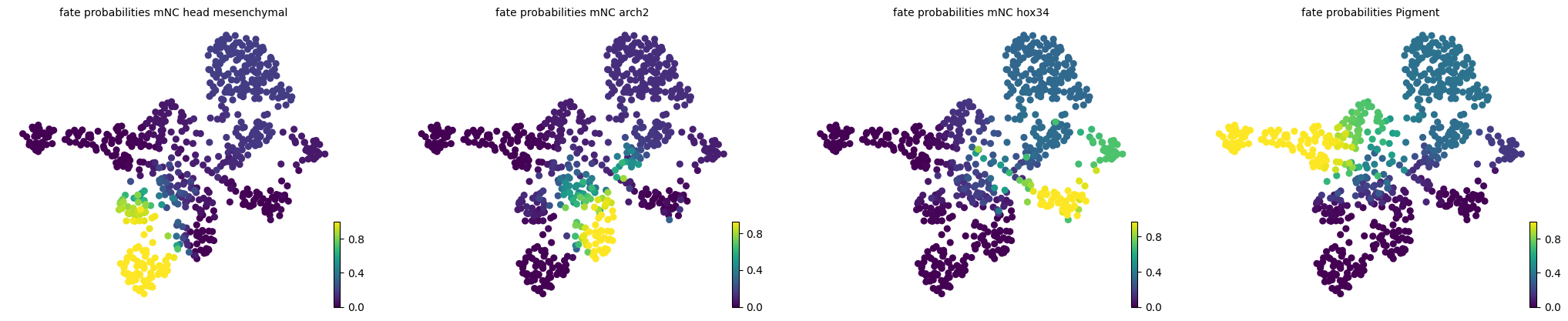
## evaluate the fate probabilities on original space
estimator.compute_macrostates(n_states=7, cluster_key="cell_type")
estimator.set_terminal_states(TERMINAL_STATES)
estimator.compute_fate_probabilities()
estimator.plot_fate_probabilities(same_plot=False)

INFO     File rgv_model/model.pt already downloaded

terminal_indices = np.where(adata.obs["term_states_fwd"].isin(TERMINAL_STATES))[0]
start_indices = np.where(adata.obs["cell_type"].isin(["NPB_nohox"]))[0]

adata_perturb, _ =  rgv.tl.in_silico_block_simulation(model=model,
                                                      adata=adata,
                                                      TF="elf1",
                                                      cutoff=0)

INFO     File rgv_model/model.pt already downloaded

vk = cr.kernels.VelocityKernel(adata).compute_transition_matrix()
vkt = vk.transition_matrix.A

vk_p = cr.kernels.VelocityKernel(adata_perturb).compute_transition_matrix()
vkt_p = vk_p.transition_matrix.A

total_simulations = rgv.tl.markov_density_simulation(adata, 
                                                     vkt, 
                                                     start_indices, 
                                                     terminal_indices, 
                                                     TERMINAL_STATES,
                                                     n_steps=500)

_ = rgv.tl.markov_density_simulation(adata_perturb, 
                                     vkt_p, 
                                     start_indices, 
                                     terminal_indices, 
                                     TERMINAL_STATES,
                                     n_steps=500)

dd_score, dd_sig = rgv.tl.simulated_visit_diff(adata, adata_perturb, TERMINAL_STATES)

rgv.pl.simulated_visit_diff(adata, 
                            adata_perturb, 
                            TERMINAL_STATES, 
                            total_simulations,
                            title="Density difference (elf1)")

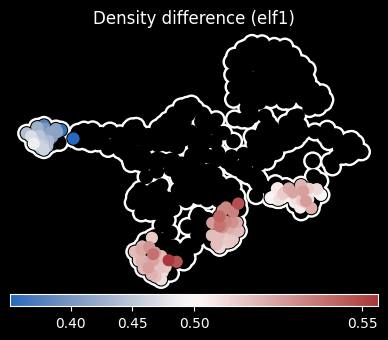
Here we can observe both depletion effects on pigment cell fate and enrichment effects on cranial mesenchyme (arch2 + facial mesenchyme) fate.

We now try to understand the underlying mechanisms.

Regulatory context of elf1

To investigate the regulatory context of elf1, we first extracted all of its downstream target genes. Specifically, we computed the global GRN and determined its downstream target genes. We then use RegVelo’s rgv.tl.regulation_scanning function to study the impact of these regulatroy edges (TF -> target gene) in our inferred GRN by systematically blocking them in silico and checking how much this changes predicted cell fates.

To zoom in the regulatory context, we firstly extracted all downstream targets of elf1. To do so, we compute the global GRN as follows:

GRN = rgv.tl.inferred_grn(vae, adata, label="cell_type", group="all", data_frame=True)

Computing global GRN...

targets = GRN.loc[:, "elf1"]
targets = np.array(targets.index.tolist())[np.array(targets) != 0]

Note

Because most gene expressions are low and noisy in single-cell context, some inferred inhibition might not be actual direct inhibition. Therefore, similar to the previous method pySCENIC, user can specifically focus on activation links via targets = np.array(targets.index.tolist())[np.array(targets) > 0]

RegVelo further screens the key regulatory link by perturbing each downstream link of elf1 and uses RegVelo depletion likelihood to rank the link, associates specific gene regulation with cell fate decision. Here we want to know which link contributes to pigment cell depletion when we remove the elf1 regulon.

perturb_screening = rgv.tl.regulation_scanning(model=model, 
                                               adata=adata, 
                                               n_states=7, 
                                               cluster_label="cell_type", 
                                               terminal_states=TERMINAL_STATES, 
                                               TF=["elf1"], 
                                               target=targets, 
                                               effect=0,
                                               n_samples=50)

INFO     File rgv_model/model.pt already downloaded
INFO     File rgv_model/model.pt already downloaded
Finished elf1 -> ENSDARG00000024966
INFO     File rgv_model/model.pt already downloaded
Finished elf1 -> ENSDARG00000042329
INFO     File rgv_model/model.pt already downloaded
Finished elf1 -> alcama
INFO     File rgv_model/model.pt already downloaded
Finished elf1 -> aopep
INFO     File rgv_model/model.pt already downloaded
Finished elf1 -> apc
INFO     File rgv_model/model.pt already downloaded
Finished elf1 -> atp6v0ca
INFO     File rgv_model/model.pt already downloaded
Finished elf1 -> baz1b
INFO     File rgv_model/model.pt already downloaded
Finished elf1 -> calr3b
INFO     File rgv_model/model.pt already downloaded
Finished elf1 -> ccny
INFO     File rgv_model/model.pt already downloaded
Finished elf1 -> cdk1
INFO     File rgv_model/model.pt already downloaded
Finished elf1 -> cdkn1ca
INFO     File rgv_model/model.pt already downloaded
Finished elf1 -> celf2
INFO     File rgv_model/model.pt already downloaded
Finished elf1 -> cenpf
INFO     File rgv_model/model.pt already downloaded
Finished elf1 -> cpeb4b
INFO     File rgv_model/model.pt already downloaded
Finished elf1 -> cxxc5b
INFO     File rgv_model/model.pt already downloaded
Finished elf1 -> diaph2
INFO     File rgv_model/model.pt already downloaded
Finished elf1 -> dlg1
INFO     File rgv_model/model.pt already downloaded
Finished elf1 -> dnajb2
INFO     File rgv_model/model.pt already downloaded
Finished elf1 -> dnmt1
INFO     File rgv_model/model.pt already downloaded
Finished elf1 -> dusp5
INFO     File rgv_model/model.pt already downloaded
Finished elf1 -> ebf3a
INFO     File rgv_model/model.pt already downloaded
Finished elf1 -> emc2
INFO     File rgv_model/model.pt already downloaded
Finished elf1 -> ephb3a
INFO     File rgv_model/model.pt already downloaded
Finished elf1 -> erbb3b
INFO     File rgv_model/model.pt already downloaded
Finished elf1 -> esco2
INFO     File rgv_model/model.pt already downloaded
Finished elf1 -> eva1ba
INFO     File rgv_model/model.pt already downloaded
Finished elf1 -> fam49a
INFO     File rgv_model/model.pt already downloaded
Finished elf1 -> fhl3a
INFO     File rgv_model/model.pt already downloaded
Finished elf1 -> fhod1
INFO     File rgv_model/model.pt already downloaded
Finished elf1 -> fli1a
INFO     File rgv_model/model.pt already downloaded
Finished elf1 -> foxo1a
INFO     File rgv_model/model.pt already downloaded
Finished elf1 -> fzd3a
INFO     File rgv_model/model.pt already downloaded
Finished elf1 -> glb1l
INFO     File rgv_model/model.pt already downloaded
Finished elf1 -> glulb
INFO     File rgv_model/model.pt already downloaded
Finished elf1 -> gpd2
INFO     File rgv_model/model.pt already downloaded
Finished elf1 -> hat1
INFO     File rgv_model/model.pt already downloaded
Finished elf1 -> hexb
INFO     File rgv_model/model.pt already downloaded
Finished elf1 -> hivep1
INFO     File rgv_model/model.pt already downloaded
Finished elf1 -> hivep3b
INFO     File rgv_model/model.pt already downloaded
Finished elf1 -> hmgn2
INFO     File rgv_model/model.pt already downloaded
Finished elf1 -> hnrnpabb
INFO     File rgv_model/model.pt already downloaded
Finished elf1 -> hpcal4
INFO     File rgv_model/model.pt already downloaded
Finished elf1 -> hsp70.2
INFO     File rgv_model/model.pt already downloaded
Finished elf1 -> hspa5
INFO     File rgv_model/model.pt already downloaded
Finished elf1 -> hspb8
INFO     File rgv_model/model.pt already downloaded
Finished elf1 -> id2a
INFO     File rgv_model/model.pt already downloaded
Finished elf1 -> ildr2
INFO     File rgv_model/model.pt already downloaded
Finished elf1 -> inka1a
INFO     File rgv_model/model.pt already downloaded
Finished elf1 -> itga3a
INFO     File rgv_model/model.pt already downloaded
Finished elf1 -> itga8
INFO     File rgv_model/model.pt already downloaded
Finished elf1 -> ivns1abpa
INFO     File rgv_model/model.pt already downloaded
Finished elf1 -> klf6a
INFO     File rgv_model/model.pt already downloaded
Finished elf1 -> kntc1
INFO     File rgv_model/model.pt already downloaded
Finished elf1 -> mbnl2
INFO     File rgv_model/model.pt already downloaded
Finished elf1 -> metrn
INFO     File rgv_model/model.pt already downloaded
Finished elf1 -> mibp
INFO     File rgv_model/model.pt already downloaded
Finished elf1 -> myo10l1
INFO     File rgv_model/model.pt already downloaded
Finished elf1 -> nr6a1b
INFO     File rgv_model/model.pt already downloaded
Finished elf1 -> pcdh2g28
INFO     File rgv_model/model.pt already downloaded
Finished elf1 -> pdgfba
INFO     File rgv_model/model.pt already downloaded
Finished elf1 -> pdlim4
INFO     File rgv_model/model.pt already downloaded
Finished elf1 -> pleca
INFO     File rgv_model/model.pt already downloaded
Finished elf1 -> plpp3
INFO     File rgv_model/model.pt already downloaded
Finished elf1 -> pmp22a
INFO     File rgv_model/model.pt already downloaded
Finished elf1 -> ppt1
INFO     File rgv_model/model.pt already downloaded
Finished elf1 -> prdm1a
INFO     File rgv_model/model.pt already downloaded
Finished elf1 -> prkceb
INFO     File rgv_model/model.pt already downloaded
Finished elf1 -> prkcsh
INFO     File rgv_model/model.pt already downloaded
Finished elf1 -> pttg1ipb
INFO     File rgv_model/model.pt already downloaded
Finished elf1 -> rabl6b
INFO     File rgv_model/model.pt already downloaded
Finished elf1 -> ralgps2
INFO     File rgv_model/model.pt already downloaded
Finished elf1 -> rgl1
INFO     File rgv_model/model.pt already downloaded
Finished elf1 -> rhbdf1a
INFO     File rgv_model/model.pt already downloaded
Finished elf1 -> rhoca
INFO     File rgv_model/model.pt already downloaded
Finished elf1 -> rxraa
INFO     File rgv_model/model.pt already downloaded
Finished elf1 -> sash1b
INFO     File rgv_model/model.pt already downloaded
Finished elf1 -> sema3d
INFO     File rgv_model/model.pt already downloaded
Finished elf1 -> sema4ba
INFO     File rgv_model/model.pt already downloaded
Finished elf1 -> sept12
INFO     File rgv_model/model.pt already downloaded
Finished elf1 -> sept9a
INFO     File rgv_model/model.pt already downloaded
Finished elf1 -> serinc5
INFO     File rgv_model/model.pt already downloaded
Finished elf1 -> shroom4
INFO     File rgv_model/model.pt already downloaded
Finished elf1 -> si:ch211-199g17.2
INFO     File rgv_model/model.pt already downloaded
Finished elf1 -> si:ch211-222l21.1
INFO     File rgv_model/model.pt already downloaded
Finished elf1 -> si:ch73-335l21.1
INFO     File rgv_model/model.pt already downloaded
Finished elf1 -> si:dkey-17m8.1
INFO     File rgv_model/model.pt already downloaded
Finished elf1 -> sipa1l2
INFO     File rgv_model/model.pt already downloaded
Finished elf1 -> slbp
INFO     File rgv_model/model.pt already downloaded
Finished elf1 -> slc12a9
INFO     File rgv_model/model.pt already downloaded
Finished elf1 -> sox6
INFO     File rgv_model/model.pt already downloaded
Finished elf1 -> src
INFO     File rgv_model/model.pt already downloaded
Finished elf1 -> stat3
INFO     File rgv_model/model.pt already downloaded
Finished elf1 -> tcf12
INFO     File rgv_model/model.pt already downloaded
Finished elf1 -> tes
INFO     File rgv_model/model.pt already downloaded
Finished elf1 -> tle3b
INFO     File rgv_model/model.pt already downloaded
Finished elf1 -> tuba8l4
INFO     File rgv_model/model.pt already downloaded
Finished elf1 -> vash2
INFO     File rgv_model/model.pt already downloaded
Finished elf1 -> vav2
INFO     File rgv_model/model.pt already downloaded
Finished elf1 -> zgc:154093
INFO     File rgv_model/model.pt already downloaded
Finished elf1 -> zgc:165573

coef = pd.DataFrame(np.array(perturb_screening["coefficient"]))
coef.index = perturb_screening["links"]
coef.columns = list(perturb_screening["coefficient"][0].keys())

We further list the top links leading to the highest pigment cell depletion.

Pigment = coef.sort_values(by="Pigment", ascending=False)[:15]["Pigment"]

df = pd.DataFrame({"Gene": Pigment.index.tolist(), "Score": np.array(Pigment)})

# Sort DataFrame by -log10(p-value) for ordered plotting
df = df.sort_values(by="Score", ascending=False)

# Highlight specific genes
# Set up the plot
with mplscience.style_context():
    sns.set_style(style="white")
    fig, ax = plt.subplots(figsize=(3, 6))
    sns.scatterplot(data=df, x="Score", y="Gene", palette="purple", s=200, legend=False)

    for _, row in df.iterrows():
        plt.hlines(row["Gene"], xmin=0.5, xmax=row["Score"], colors="grey", linestyles="-", alpha=0.5)

    # Customize plot appearance
    plt.xlabel("Pigment depletion likelihood")
    plt.ylabel("")
    plt.title("Pigment")

    plt.gca().spines["top"].set_visible(False)
    plt.gca().spines["right"].set_visible(False)
    plt.gca().spines["left"].set_color("black")
    plt.gca().spines["bottom"].set_color("black")
    # Show plot

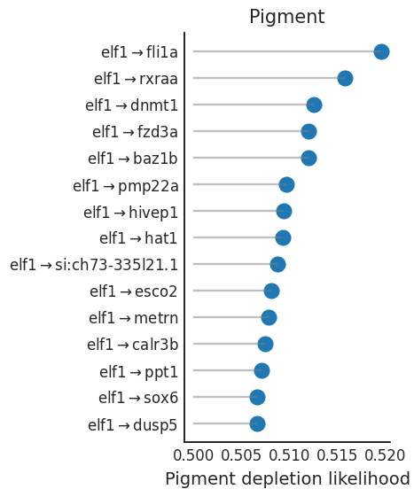
We see that elf1 -> fli1a is ranked as the top link affecting pigmentation. We further focus on the upstream of elf1 to study which regulators determine the elf1 expression in driving pigmentation.

regulators = GRN.loc["elf1",:]
regulators = np.array(regulators.index.tolist())[np.array(regulators) != 0]

perturb_screening_tf = rgv.tl.regulation_scanning(model=model, 
                                                  adata=adata, 
                                                  n_states=7, 
                                                  cluster_label="cell_type", 
                                                  terminal_states=TERMINAL_STATES, 
                                                  TF=regulators, 
                                                  target=["elf1"], 
                                                  effect=0,
                                                  n_samples=50)

INFO     File rgv_model/model.pt already downloaded
INFO     File rgv_model/model.pt already downloaded
Finished arntl1b -> elf1
INFO     File rgv_model/model.pt already downloaded
Finished fli1a -> elf1
INFO     File rgv_model/model.pt already downloaded
Finished fosl2 -> elf1
INFO     File rgv_model/model.pt already downloaded
Finished hnf1ba -> elf1
INFO     File rgv_model/model.pt already downloaded
Finished hoxa4a -> elf1
INFO     File rgv_model/model.pt already downloaded
Finished hoxb8a -> elf1
INFO     File rgv_model/model.pt already downloaded
Finished hoxc3a -> elf1
INFO     File rgv_model/model.pt already downloaded
Finished sox10 -> elf1
INFO     File rgv_model/model.pt already downloaded
Finished sox9b -> elf1
INFO     File rgv_model/model.pt already downloaded
Finished tfap2a -> elf1
INFO     File rgv_model/model.pt already downloaded
Finished tfec -> elf1

coef = pd.DataFrame(np.array(perturb_screening_tf["coefficient"]))
coef.index = perturb_screening_tf["links"]
coef.columns = list(perturb_screening_tf["coefficient"][0].keys())

Pigment = coef.sort_values(by="Pigment", ascending=False)["Pigment"]

df = pd.DataFrame({"Gene": Pigment.index.tolist(), "Score": np.array(Pigment)})

# Sort DataFrame by -log10(p-value) for ordered plotting
df = df.sort_values(by="Score", ascending=False)

# Highlight specific genes
# Set up the plot
with mplscience.style_context():
    sns.set_style(style="white")
    fig, ax = plt.subplots(figsize=(4, 6))
    sns.scatterplot(data=df, x="Score", y="Gene", palette="purple", s=200, legend=False)

    for _, row in df.iterrows():
        plt.hlines(row["Gene"], xmin=0.45, xmax=row["Score"], colors="grey", linestyles="-", alpha=0.5)

    # Customize plot appearance
    plt.xlabel("Pigment depletion likelihood")
    plt.ylabel("")
    plt.title("Pigment")

    plt.gca().spines["top"].set_visible(False)
    plt.gca().spines["right"].set_visible(False)
    plt.gca().spines["left"].set_color("black")
    plt.gca().spines["bottom"].set_color("black")
    # Show plot

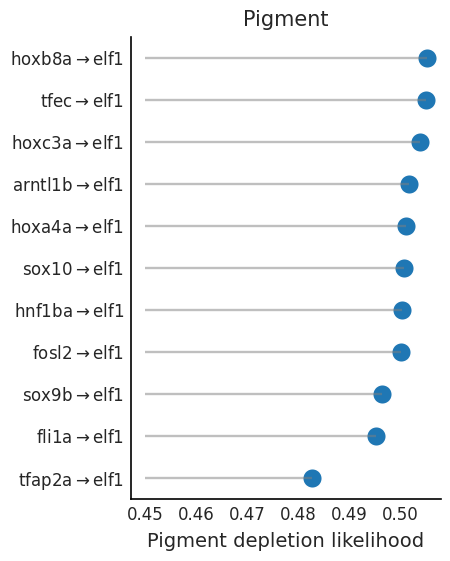
We see that hoxb8a and tfec are the top regulators of elf1. We have now found a subnetwork centered around elf1 for the pigment cell fate determination.

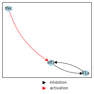
Visualization of the genetic circuit

We further visualize this genetic circuit, in which we include its top upstream regulator tfec and downstream target fli1a.

motif = [
    ["tfec","elf1", GRN.loc["elf1","tfec"]],
    ["elf1", "fl1a", GRN.loc["elf1", "fli1a"]],
    ["fl1a", "elf1", GRN.loc["fli1a", "elf1"]],
]

motif = pd.DataFrame(motif)

motif.columns = ["from", "to", "weight"]
motif["weight"] = np.sign(motif["weight"])

with mplscience.style_context():
    rgv.pl.regulatory_network(motif=motif)

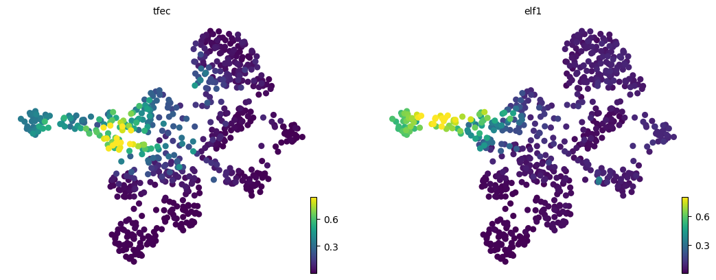
Visualization genetic circut

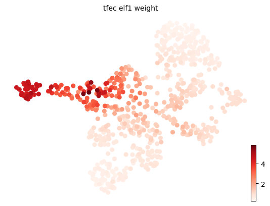
Using the Jacobian matrix framework [Qiu et al., 2022], RegVelo also enables the estimation of cell-specific regulatory weights. We can easily visualize this in a 2D embedding space. In the following, we demonstrate this for the regulatory edge tfec -> elf1.

GRN = rgv.tl.inferred_grn(vae, adata, cell_specific_grn=True)

GRN.shape

(697, 1008, 1008)

Note

The estimated cell-specific GRN has three dimensions: the first corresponds to the cells, the second to the target genes, and the third to the regulator genes.

tfec_elf1 = GRN[:,[i == "elf1" for i in adata.var.index], [i == "tfec" for i in adata.var.index]].reshape(-1)

adata.obs["tfec_elf1_weight"] = tfec_elf1

scv.pl.umap(adata,
            color=["tfec","elf1"],
            frameon=False,layer = ["Ms"],title = ["tfec","elf1"])

scv.pl.umap(adata,
            color=["tfec_elf1_weight"],
            cmap="Reds")