Application: Model selection on mouse neural crest and schwann cell dataset
In this notebook, we will use the ModelComparison class from regvelo to select an optimal model setup based on the real time and the stemness score. Using the best-performing model, we further perform a trajectory and latent time prediction. The dataset used in this notebook is a subset of the dataset used in Kastriti, M. E. et al, 2022. It consists of Smart-seq2 single-cell transcriptomes from mouse cells spanning embryonic to adult stages and covering the full neural crest lineage, including Schwann cell precursors.
A detailed tutorial on how to use RegVelo’s ModelComparison class is provided in the Model Comparison Tutorial.
Library import
import numpy as np
import scanpy as sc
import cellrank as cr
import scvi
import scvelo as scv

import regvelo as rgv
from regvelo import REGVELOVI
from regvelo import ModelComparison
General settings and function definition
scvi.settings.seed = 0
scv.settings.set_figure_params("scvelo", dpi=80, transparent=True, fontsize=14, color_map="viridis")
%matplotlib inline
def min_max_scaling(data):
    """Compute min and max values for each feature."""
    min_vals = np.min(data, axis=0)
    max_vals = np.max(data, axis=0)

    # Perform min-max scaling
    scaled_data = (data - min_vals) / (max_vals - min_vals)

    return scaled_data
Load data
In the following, we load the preprocessed mouse neural crest dataset and define the true developmental time and save it to adata.obs["devtime"].
adata = rgv.datasets.schwann()
## convert developmental time as integer values
mapping = {
    "E9.5": 0, "E10.5": 1, "E11.5": 2, "E12.5": 3, "E13.5": 4,
    "E14.5": 5, "E16.5": 6, "E18.5": 7, "P0": 8, "P2": 9,
    "P6": 10, "P10": 11, "Adult": 12
}

adata.obs["devtime"] = adata.obs["devtime"].astype(str).replace(mapping).astype(np.float32)
adata
AnnData object with n_obs × n_vars = 8821 × 1150
    obs: 'plates', 'devtime', 'location', 'n_genes_by_counts', 'total_counts', 'total_counts_ERCC', 'pct_counts_ERCC', 'doublet_scores', 'leiden', 'CytoTRACE', 'Gut_neuron', 'Sensory', 'Symp', 'enFib', 'ChC', 'Gut_glia', 'NCC', 'Mesenchyme', 'Melanocytes', 'SatGlia', 'SC', 'BCC', 'conflict', 'assignments', 'batch', 'initial_size_unspliced', 'initial_size_spliced', 'initial_size', 'n_counts'
    var: 'ERCC', 'n_cells_by_counts', 'mean_counts', 'pct_dropout_by_counts', 'total_counts', 'n_cells', 'm', 'v', 'n_obs', 'res', 'lp', 'lpa', 'qv', 'highly_variable', 'Accession', 'Chromosome', 'End', 'Start', 'Strand', 'TF', 'means', 'dispersions', 'dispersions_norm', 'velocity_genes'
    uns: 'assignments_colors', 'devtime_colors', 'hvg', 'leiden', 'leiden_colors', 'leiden_sizes', 'location_colors', 'log1p', 'neighbors', 'network', 'paga', 'regulators', 'skeleton', 'targets', 'umap'
    obsm: 'X_diff', 'X_pca', 'X_umap'
    layers: 'GEX', 'Ms', 'Mu', 'ambiguous', 'matrix', 'palantir_imp', 'scaled', 'spanning', 'spliced', 'unspliced'
    obsp: 'connectivities', 'distances'
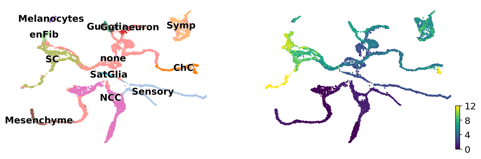
scv.pl.scatter(adata, basis="umap", title="", color=["assignments","devtime"], legend_loc="on data")
ModelComparison
Object initialization
We now initialize the ModelComparison object.
comp = ModelComparison(adata = adata)
Train
We set batch_size to np.min(adata.shape[0], 5000) to avoid out of memory issue.
comp.train(model_list=['soft','hard','soft_regularized'],
           lam2=[1.0],
           n_repeat=1,
           batch_size=min(adata.shape[0], 5000))
Epoch 1369/1500:  91%|█████████▏| 1369/1500 [45:44<04:22,  2.01s/it, v_num=1]
Monitored metric elbo_validation did not improve in the last 45 records. Best score: -4881.255. Signaling Trainer to stop.
Epoch 1424/1500:  95%|█████████▍| 1424/1500 [46:44<02:29,  1.97s/it, v_num=1]
Monitored metric elbo_validation did not improve in the last 45 records. Best score: -4652.919. Signaling Trainer to stop.
Epoch 1050/1500:  70%|███████   | 1050/1500 [35:02<15:00,  2.00s/it, v_num=1]
Monitored metric elbo_validation did not improve in the last 45 records. Best score: -3928.337. Signaling Trainer to stop.
['soft_0', 'hard_0', 'soft_regularized\nlam2:1.0_0']
Evaluate and save
We evaluate the model performance based on the real developmental time and how well the model preserves undifferentiated cell states.
# Based on real developmental time
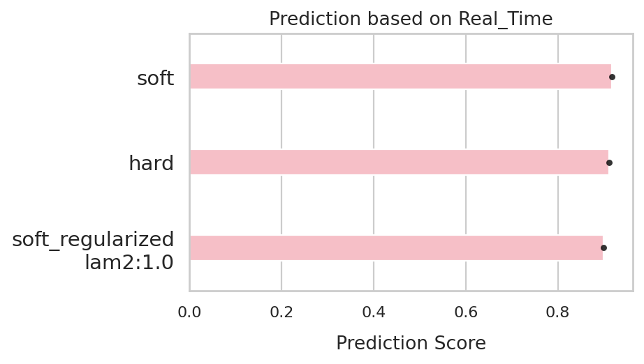
comp.evaluate(side_information='Real_Time',
side_key = 'devtime')
('df_Real_Time',
                         Model      Corr Run
 0                        soft  0.917364   0
 1                        hard  0.910931   0
 2  soft_regularized\nlam2:1.0  0.898595   0)
comp.plot_results(side_information='Real_Time')
# Based on stemness score
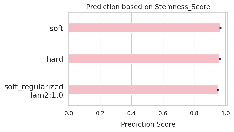
comp.evaluate(side_information='Stemness_Score',
side_key='CytoTRACE')
('df_Stemness_Score',
                         Model      Corr Run
 0                        soft  0.964955   0
 1                        hard  0.960132   0
 2  soft_regularized\nlam2:1.0  0.948968   0)
comp.plot_results(side_information='Stemness_Score')
comp.MODEL_TRAINED
REGVELOVI Model with the following params:
n_hidden: 256, n_latent: 10, n_layers: 1, dropout_rate: 0.1
Training status: Trained
REGVELOVI Model with the following params:
n_hidden: 256, n_latent: 10, n_layers: 1, dropout_rate: 0.1
Training status: Trained
REGVELOVI Model with the following params:
n_hidden: 256, n_latent: 10, n_layers: 1, dropout_rate: 0.1
Training status: Trained
{'soft_0': , 'hard_0': , 'soft_regularized\nlam2:1.0_0': }
vae_s = comp.MODEL_TRAINED['soft_0']
vae_s.save('vae_s')
Trajectory and latent time prediction
vae_s = REGVELOVI.load('vae_s', adata)
rgv.tl.set_output(adata, vae_s, n_samples=30, batch_size=5000)
INFO File vae_s/model.pt already downloaded
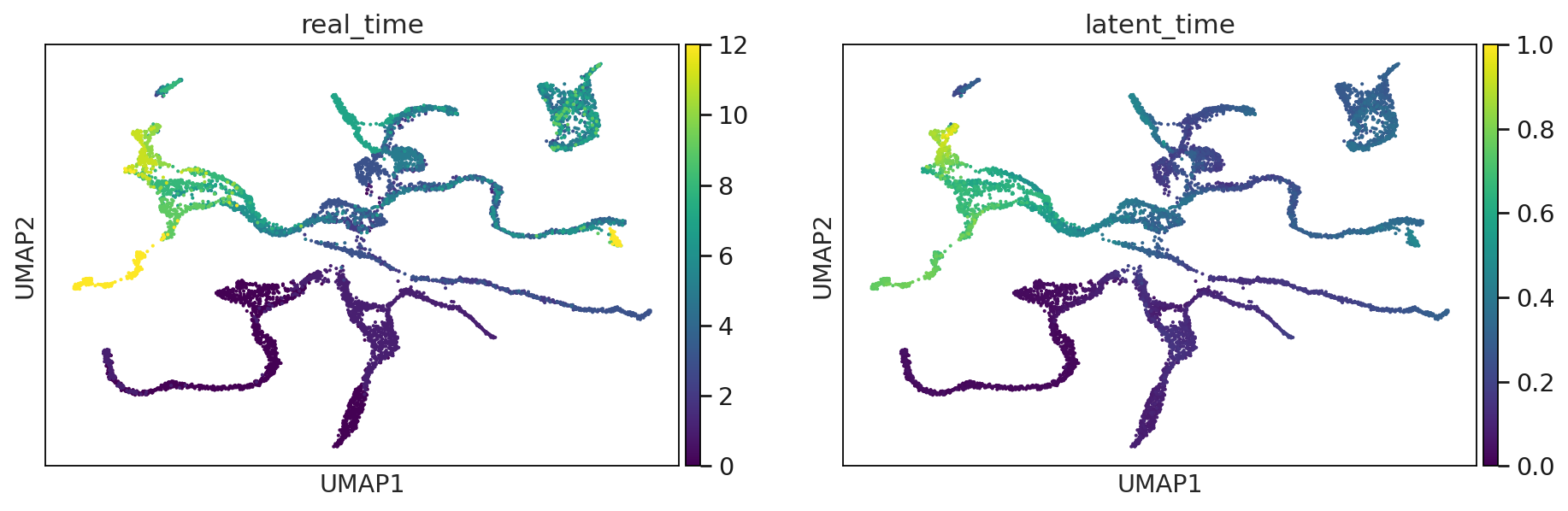
adata.obs["latent_time"] = min_max_scaling(adata.layers["fit_t"].mean(1))
scv.settings.set_figure_params("scvelo", dpi=80, transparent=True, fontsize=14, color_map="viridis")
sc.pl.umap(adata, title=["real_time", "latent_time"],color = ["devtime", "latent_time"], legend_loc="on data")
scv.tl.velocity_graph(adata)
computing velocity graph (using 1/128 cores)
    finished (0:00:07) --> added
    'velocity_graph', sparse matrix with cosine correlations (adata.uns)
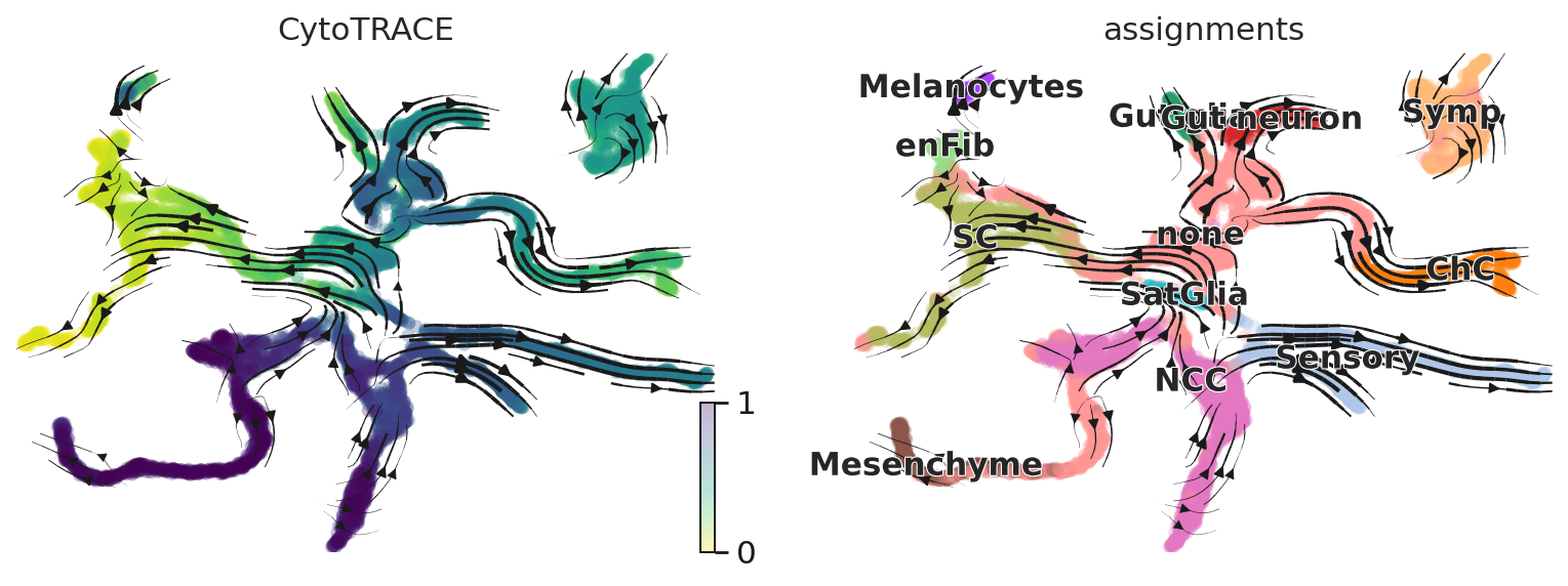
scv.pl.velocity_embedding_stream(adata, basis="umap", color=["CytoTRACE", "assignments"])
computing velocity embedding
    finished (0:00:01) --> added
    'velocity_umap', embedded velocity vectors (adata.obsm)